A drop checker is a brilliant addition to a CO2 gas-injected planted aquarium and is an equilibrium method for reading out the amount of dissolved CO2 in the water column. Drop checkers rely on the pH indicator bromothymol blue in a solution of 4 dKH alkalinity . ‘Hoppy’ (Vaughn Hopkins) popularised the mechanistic underpinnings of the chemistry to the hobby in late 2006 and the concept spread rapidly in online forums like Aquatic Plant Central and the Barr Report. Hoppy pointed out: “The reason for setting the KH of the indicator solution to 4 is so that with 30 ppm of CO2 the indicator color will be green, and an unequivocal green.”
Unequivocal green
…and that’s the problem. When a 4 dKH drop checker is “green”, how green is that?
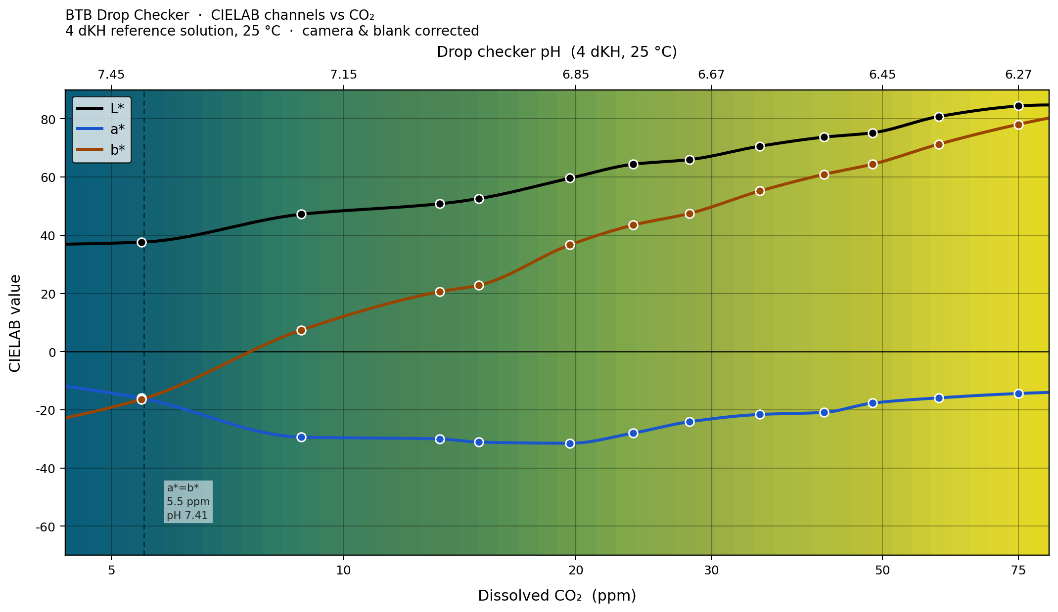
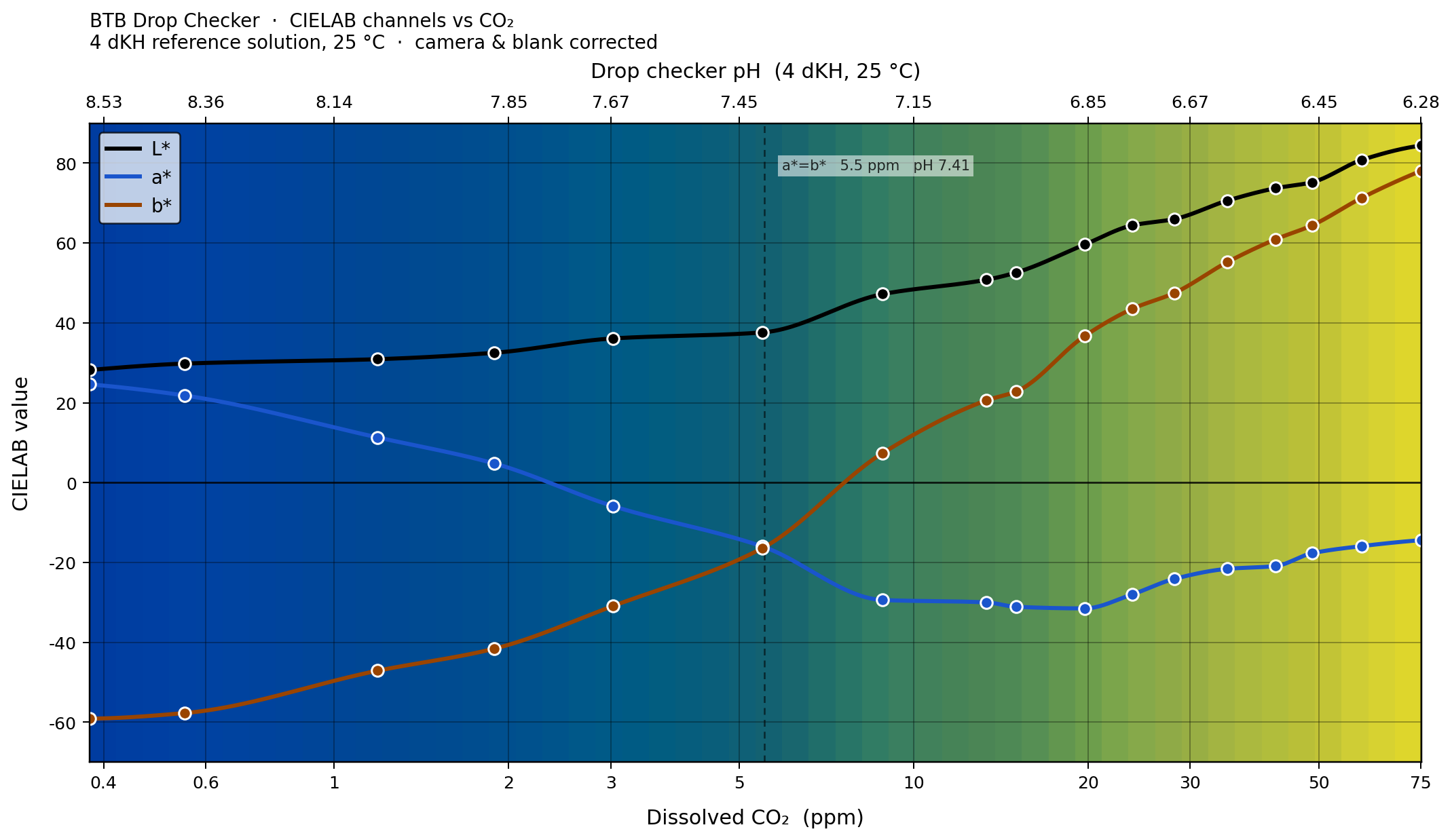
Bromothymol blue calibrated colour vs. aquarium dissolved CO2 concentration
Above is a colour calibrated dataset that shows the colour of a 4 dKH drop checker vs. dissolved CO2 concentration in the aquarium. Also shown are the numerical CIELAB perceptual values for L* (luminosity), a* (green-red axis) and b* (blue-yellow axis). The colours are calibrated against a standard D65 illuminant, which is roughly what overcast daylight seen indoors through a north-facing window from somewhere in Europe would look like.
The blue-green-yellow colour of a drop checker comes from the pH-sensitive dye bromothymol blue (BTB) in a solution of 4.0 dKH water. There is an exact correspondence between the level of CO2 in the aquarium and the equilibrium pH inside the drop checker that the BTB experiences. You can read off the pH inside the drop checker from the top X-axis of the figure as well. Note that the drop checker takes about 2 hours to align the CO2 concentration in the drop checker solution with the CO2 concentration in the water.
Making a calibrated BTB colour dataset
This turns out to be not at all straightforward… There are two main challenges:
Ensuring the reference solutions have accurate pH and ionic strength
Image capture and analysis that normalises raw data in perceptual space into standard illuminant conditions
Raw colour dataset acquired in defined pH conditions
water blank - pH 8.56
pH 8.56
pH 8.40
pH 8.07
pH 7.87
pH 7.67
pH 7.41
pH 7.20
pH 7.03
pH 6.97
pH 6.86
pH 6.77
pH 6.70
pH 6.61
pH 6.53
pH 6.46
pH 6.38
pH 6.28
Reference solutions for BTB colour assessment
Importance of defining pH and ionic strength
BTB exists in an equilibrium between two different pH-sensitive chemical forms – one which “looks blue” and the other which “looks yellow”. The relative amount of these two forms in a solution of a given pH can be described by BTB’s pKa – when pH equals pKa there is an equal representation of both forms. As pH shifts up or down from the pKa the relative amounts change* and that affects the perceptual colour of the solution. That means we need to be able to accurately set the pH of test solutions to measure the visual characteristics of BTB.
We also have to set the ionic strength (salt concentration) at something suitable. Drop checker standard dKH of 4.0 might sound like a big number but it’s actually pretty close to distilled water as these things go. For reference, standard seawater has about 700 mM “salt” where the 4.0 dKH solution is only 1.4 mM “salt”. We need to stay in the low single-digit mM salt range for calibrated BTB colour measurements because salt changes the way BTB interacts with acidity – the Debye-Hückel effect – and if things get “too salty” the colour dependence of BTB on pH starts changing. This “stay at low salt” consideration also means a lot of the scientific literature around BTB the hobby would otherwise like to use doesn’t properly apply to drop checkers. It turns out that BTB is not very soluble in pure water so a lot of the ‘sci-lab’ experiments are done at 100 mM salt and that is a level of salt that materially changes BTB’s colour properties. Similarly, many of the commonly used ‘sci-lab’ methods for making defined pH solutions, e.g. relative ratio mixtures of KH2PO4 and K2HPO4, are also done at 100+ mM salt concentrations and won’t do a good job of modeling a drop checker’s pH-colour dependence.
Making known pH and ionic strength BTB solutions
We’re going to mix three well-defined solutions to create conditions suitable for measuring BTB colouration.
BTB stock solution
10 dKH water
30 mM HCl
13.73 g distilled water
1) make 400 dKH water by adding 1.20 g baking soda to 99.4 g distilled water
3.06 g 1M HCl
13.73 g 100% methanol
2) mix 2.5 g 400 dKH water with 97.5 g distilled water
97.0 g distilled water
0.030 g BTB (sodium salt)
0.1% BTB 50/50 w/w MeOH/H2O
serial dilution method
note: density of 1M HCl is 1.02 g/ml
The overall concept is to start with 10 dKH water in a cuvette, add a suitable amount of BTB solution and then reduce the pH to something suitable by adding a quantified aliquot of hydrochloric acid (HCl). The HCl will react essentially instantaneously with the bicarbonate (HCO3–) in the 10 dKH water, converting bicarbonate to composite carbonic acid (CO2*). We start with 10 dKH water in the reaction because this is low enough ionic strength to not need any Debye-Hückel effect correction, yet high enough that there will still be some carbonate alkalinity remaining after addition of the HCl. The BTB solution (water/methanol) contributes no alkalinity. We will account for the dilution effects of both the BTB dye and the HCl to the total volume of the reaction.
Importantly, we do not need to measure the pH of the test solution in the cuvette – we will instead determine the pH analytically from first principles. This first principles derivation involves the full carbonate system charge balance and all its polynomial forms #. The only physical constants needed are the ionisation constant of water (Kw), and the pKa of composite carbonic acid (K1 – transition to bicarbonate) and the pKa of bicarbonate (K2 – transition to carbonate) all of which are very well established. We do NOT need to know the pKa of BTB. Knowing total solution volume, volume-adjusted dKH and amount of HCl we can solve for [H+] and thereby for pH since pH = -log10[H+]. The charge balance equation, which is quartic in [H+], is solved numerically (python coded example given below).
Temperature considerations
Temperature does affect the colour characteristics of BTB, but generally not enough to make a meaningful difference vs the effect from pH. You do not need to worry that the temperature of the aquarium where your drop checker lives might not be the same as where you calibrated the colour readings. Adding acid to bicarbonate also formally liberates a small amount of heat; again not enough to make a meaningful difference. The one thing you do need to be careful with though is that the choice of constants for Kw, K1 and K2 that go into the pH calculations are sensitive to temperature – you need to use constants that match the temperature at which you take calibrated BTB colour readings (generally this will be room temperature).
Work quickly – this is a non-equilibrium method
Best is to pre-mix 10 dKH water with BTB solution. If you upscale from 0.1 g BTB stock solution added to 5.0 g 10 dKH water, you get a solution that is just under 20 ppm BTB which is a good concentration well representative of commercial drop checker dye concentrations. The additional dilution of the dye from the volume component of the of added HCl doesn’t shift the colour of BTB – only a slight decrease in saturation. The reduction in pH caused by the acid component of the added HCl will of course have a dramatic effect on the BTB apparent colour.
“Quickly” in this context means add the acid, do a gentle swirl to get complete mixing, position the cuvette and take the photograph. Then discard the solution. Before the acid is added, all three of the 10 dKH water, BTB dye stock solution and the 30 mM HCl are equilibrated to typical indoor CO2 concentrations. In my case, indoor CO2 in our not-very-well-insulated cottage is usually between 600 to 700 ppm (we have an indoor CO2 monitor which measures this), which by Henry’s Law means solutions will equilibrate to around 1 ppm dissolved CO2. Those solutions are all stable. After the acid is added it instantly converts bicarbonate to composite carbonic acid – this is what sets the pH in the cuvette and thereby also the colour of the BTB. Elevated composite carbonic acid however is NOT stable. The CO2 form will straight away start outgassing from the cuvette to restore CO2 equilibrium with atmosphere. If you let the cuvette stand you can see this happening in real time – over the course of 5 or 10 minutes you’ll see a blue layer appear on the surface of an otherwise more yellowish solution – this is the pH at the liquid surface rising from escaped CO2 and the associated BTB colour change in that region. For this reason, doing serial additions of acid – add some acid, mix and photograph, then add a little more acid, mix and photograph – is not a good idea. Loss of CO2 due to outgassing will systematically mean the solution pH is higher than you would otherwise calculate it to be under this serial acid addition approach.
Capturing and quantifying the perceptual colour of BTB solutions
Standardised lighting and camera setup
It is important to have uniformity in the both the lighting and camera setup when capturing and analysing images of well-defined pH BTB solutions. I use an overhead ring light above the sample cuvette to prevent shadows. Background is a neutral white piece of paper. The cuvette is mounted on a stable surface at a defined height. I used a Pixel 8 mobile phone as the camera, also mounted on a stable stand. There are some good apps that will let you take a time-lapse series of photographs, all locked to the same focus, exposure and white balance. I like Velocity Lapse – easy to use with a good, intuitive interface. Be sure your pictures capture both the cuvette and a region of neutral white background outside the cuvette. Include a photograph of a cuvette ‘blank’ – liquid but no dye – in your image series.
Colour quantification and correction
Colour measurements were extracted from smartphone images using a 50 × 50 px colour picker tool in GIMP, directly reporting CIELAB values. For each sample (including the blank) the central bulk area of the solution in the cuvette was measured, as was an area of neutral white background outside the cuvette. CIELAB isn’t linear in the way we need for optical correction, so these values were converted to CIE XYZ tristimulus values, which are linear in light intensity and therefore suitable for ratio-based optical correction.
Colour correction proceeded in two steps. First, each image’s XYZ values were normalised to that image’s white background measurement, removing per-photograph illumination and white balance variation. Second, the water blank — itself white-corrected — was used to remove the multiplicative contributions of the cuvette optics and camera spectral response by channel-wise division by the blank’s XYZ values. The resulting XYZ values were then rescaled to the D65 standard white point and converted back to CIELAB. The water blank corrects to L*=100, a*=0, b*=0, confirming the correction is working as expected.
Standardised BTB colour vs reference pH
The output of the overall workflow is a matched relationship between pH and BTB perceptual colour. With a reasonable number of data pairs across the expected pH range it is straightforward to interpolate observed colour in the drop checker with the pH in the drop checker that is causing that perceived colour. With the now known drop checker pH (inferred by colour) and the prespecified drop checker dKH (usually 4.0) a related first principles derivation can output the concentration of CO2 inside the drop checker, and thereby also inside the aquarium.
All low CO2 levels look dark blue
Results from the full workflow reveal an interesting fact about BTB as a drop checker indicator. There is a lot of differential CIELAB movement at CO2 levels < 5 ppm which is where you might expect a non-CO2 injected aquarium to run. Almost none of that makes an actual perceptual difference however – everything just looks ‘dark blue’.
Bromothymol blue calibrated colour vs. aquarium dissolved CO2 concentration
Notes:
* The relative fractions of the two forms at a given pH are broadly described by the Henderson-Hasselbalch (H-H) equation. We don’t actually use the H-H equation because H-H requires total alkalinity be attributable solely to bicarbonate, and this assumption breaks down under some of the lower pH conditions we’ll be assessing.
# Stumm, W. and Morgan, J.J. (1996) Aquatic Chemistry: Chemical Equilibria and Rates in Natural Waters, 3rd edition. Wiley, New York.
Python code to solve for pH, remaining dKH and [CO2*]
Copy and paste into Colab. Substitute your own values into the # ── PARAMETERS and # ── TITRATION ROWS sections.
import numpy as np
import pandas as pd
from scipy.optimize import brentq

# Closed-system carbonate titration simulator
# ------------------------------------------
# This version treats the three input solutions separately:
#   1) starting water: known TA from dKH, baseline dissolved CO2
#   2) dye stock:      TA ~ 0, baseline dissolved CO2
#   3) acid stock:     TA = -[HCl], baseline dissolved CO2
#
# It then mixes them in a CLOSED system (no CO2 exchange with air),
# solves the final carbonate equilibrium from TA and CT, and reports
# pH, dKH, and dissolved CO2 (ppm as CO2).

# ── CONSTANTS (20°C, freshwater, I=0) ────────────────────────────────────────
K1 = 4.16e-7
K2 = 4.20e-11
Kw = 6.81e-15

# ── PARAMETERS ───────────────────────────────────────────────────────────────
KH0_dKH  = 10.0    # starting alkalinity of water (dKH)
ca_mM    = 30.0    # acid concentration (mM)
CO2a_ppm = 1.000   # dissolved CO2 in starting water, dye stock, and acid stock (ppm)

# ── TITRATION ROWS ───────────────────────────────────────────────────────────
# Paste tab- or space-separated values: Vwater_mL  Vdye_mL  Vacid_mL
# One row per line. Header line is ignored if present.
titration_data = """
Vwater  Vdye    Vacid
5	0.1	0.055
5	0.1	0.082
5	0.1	0.114
5	0.1	0.125
5	0.1	0.153
5	0.1	0.175
5	0.1	0.196
5	0.1	0.224
5	0.1	0.251
5	0.1	0.272
5	0.1	0.301
5	0.1	0.336
"""

# ── UNIT CONVERSIONS ─────────────────────────────────────────────────────────
def dkh_to_eq(dkh):
    return dkh * 0.000357  # eq/L

def eq_to_dkh(eq):
    return eq / 0.000357

def ppm_to_mol(ppm):
    return ppm / 44010.0   # mol/L, as CO2

def mol_to_ppm(mol):
    return mol * 44010.0

# ── CARBONATE SOLVER ─────────────────────────────────────────────────────────
def solve_h(TA, CT):
    """
    Solve for [H+] from total alkalinity (eq/L) and total inorganic carbon (mol/L).

    TA = [HCO3-] + 2[CO3--] + [OH-] - [H+]
    CT = [CO2*] + [HCO3-] + [CO3--]
    """
    def f(h):
        denom  = h**2 + K1*h + K1*K2
        alpha1 = (K1 * h)  / denom   # fraction as HCO3-
        alpha2 = (K1 * K2) / denom   # fraction as CO3--
        return h + TA - CT*(alpha1 + 2*alpha2) - Kw/h

    return brentq(f, 1e-14, 1.0)

def co2_star(CT, h):
    """Return dissolved CO2* from CT and [H+]."""
    denom = h**2 + K1*h + K1*K2
    return CT * h**2 / denom

def ct_from_ta_and_co2star(TA, co2_star_baseline):
    """
    Given TA and a specified dissolved CO2* baseline, solve the stock equilibrium
    and return CT.
    """
    def f(h):
        return h + TA - K1*co2_star_baseline/h - 2*K1*K2*co2_star_baseline/h**2 - Kw/h

    # Wide bracket works for water, neutral-ish dye stock, and acidic stock
    h = brentq(f, 1e-14, 1.0)
    ct = co2_star_baseline * (h**2 + K1*h + K1*K2) / h**2
    return h, ct

# ── SIMULATION ───────────────────────────────────────────────────────────────
def simulate_titration(rows, KH0_dKH, ca_mM, CO2a_ppm):
    ta_water     = dkh_to_eq(KH0_dKH)
    co2_baseline = ppm_to_mol(CO2a_ppm)
    ca_eq_per_L  = ca_mM * 1e-3  # mol/L HCl = eq/L acid

    # Starting solution equilibria
    h_w, ct_water = ct_from_ta_and_co2star(ta_water,      co2_baseline)
    h_d, ct_dye   = ct_from_ta_and_co2star(0.0,           co2_baseline)
    h_a, ct_acid  = ct_from_ta_and_co2star(-ca_eq_per_L,  co2_baseline)

    results = []
    for (Vw, Vd, Va) in rows:
        Vf = (Vw + Vd + Va) / 1000.0  # L

        # TA moles: water contributes positive TA, acid subtracts TA
        ta_mol = ta_water * Vw/1000.0 - ca_eq_per_L * Va/1000.0

        # CT moles: each stock contributes its own equilibrium CT
        ct_mol = (
            ct_water * Vw/1000.0 +
            ct_dye   * Vd/1000.0 +
            ct_acid  * Va/1000.0
        )

        ta_f = ta_mol / Vf
        ct_f = ct_mol / Vf

        h_f     = solve_h(ta_f, ct_f)
        ph_f    = -np.log10(h_f)
        co2_out = mol_to_ppm(co2_star(ct_f, h_f))
        dkh_out = eq_to_dkh(ta_f)

        results.append({
            "Va_mL":     round(Va, 3),
            "pH":        round(ph_f, 3),
            "dKH":       round(dkh_out, 3),
            "CO2_ppm":   round(co2_out, 4),
            "CT_mM":     round(ct_f * 1000.0, 5),
            "TA_meq_L":  round(ta_f * 1000.0, 5),
        })

    return pd.DataFrame(results), {
        "pH_water": -np.log10(h_w),
        "pH_dye":   -np.log10(h_d),
        "pH_acid":  -np.log10(h_a),
        "CT_water_mM": ct_water * 1000.0,
        "CT_dye_mM":   ct_dye * 1000.0,
        "CT_acid_mM":  ct_acid * 1000.0,
    }

# ── PARSE INPUT ───────────────────────────────────────────────────────────────
rows = []
for line in titration_data.strip().splitlines():
    parts = line.split()
    if not parts or not parts[0].replace('.', '').replace('-', '').isdigit():
        continue
    rows.append((float(parts[0]), float(parts[1]), float(parts[2])))

# ── RUN ───────────────────────────────────────────────────────────────────────
df, stock_info = simulate_titration(rows, KH0_dKH, ca_mM, CO2a_ppm)

print("Stock equilibria")
for k, v in stock_info.items():
    print(f"{k}: {v:.6f}")
print()
print(df.to_string(index=False))